High-Precision Audio Drift Measurements with GPS
-
 Mario Guggenberger
 - August 20, 2015
This guide will guide you through instructions on how to conduct high-precision audio drift and frequency measurements with an ordinary desktop PC or laptop.
Contents
- Introduction
- Requirements
- Setup
- Measuring Playback Drift
- Measuring Recording Drift
- Measuring Frequency
- Example Measurements
- Troubleshooting
- Resources
Introduction
Drifts in ADCs and DACs of audio interfaces are usually very low and detecting and measuring them requires precise equipment, which is usually extremely expensive and therefore very rarely available. Measuring the drift can either be done directly on the hardware level by measuring the clock generator on the circuitry, or more easily by treating the target device or system as a black box and working with its input and output. The latter case is what this guide focuses on.
Measuring the ADC drift basically works by feeding the device a frequency-calibrated analog signal and determining from the recorded digital samples how much the recorded frequency differs from the fed (nominal) frequency, and the drift is then simply a function of the difference between the nominally expected and the recorded frequency of the signal. Measuring the DAC works the other way round by playing back a digital signal with the nominal frequency and measuring the frequency of the analog output with a calibrated frequency meter or frequency counter, where the drift is again a function of the expected and measured frequency.
What makes this endeavor expensive is the need for a calibrated high-precision frequency counter that can measure frequencies and output calibrated test signals. There are various devices available on the market, e.g. from Agilent / Keysight Technologies, that can cost thousands of Euros. They are driven by very precise clock generators, usually atomic clocks. To save this money, another already ubiquitous technology that needs precise timing to function correctly can be used: GPS, which we are going to exploit to turn a regular computer into a cheap but precise frequency counter.
A GPS receiver basically calculates its position by measuring the time that signals from multiple satellites, which each carries multiple atomic clocks, take to arrive at the receiver. The more precise the timing information from satellites is, the more accurate is the calculated position. This means that the GPS system strives to maintain as precise timing information as possible, which is the reason why it is a very good timing source that is free for anyone to use and used in many applications. According to The Science of Timekeeping, a GPS time stamp is theoretically accurate to 14 nanoseconds. The accuracy of the GPS receiver that we are going to use is specified at 1 µs, which is still accurate enough to measure even tiny drifts in multimedia devices or to measure the influence of the environmental temperature on the drift.
The system that we are going to build works like this: A computer runs the Spectrum Lab audio spectrum analyzer software to analyze a stereo input signal sampled by the audio interface. The stereo input consists of a GPS time pulse signal in one channel and the signal to be measured in the other channel. Because the computer used for this measurement is also prone to drift, Spectrum Lab takes the GPS time signal as its non-drifted precise time base instead of the drifted computer time base to measure the absolute drift in the input signal. All of the required files referred to in this guide are either linked to or available in the accompanying GitHub repository.
Requirements
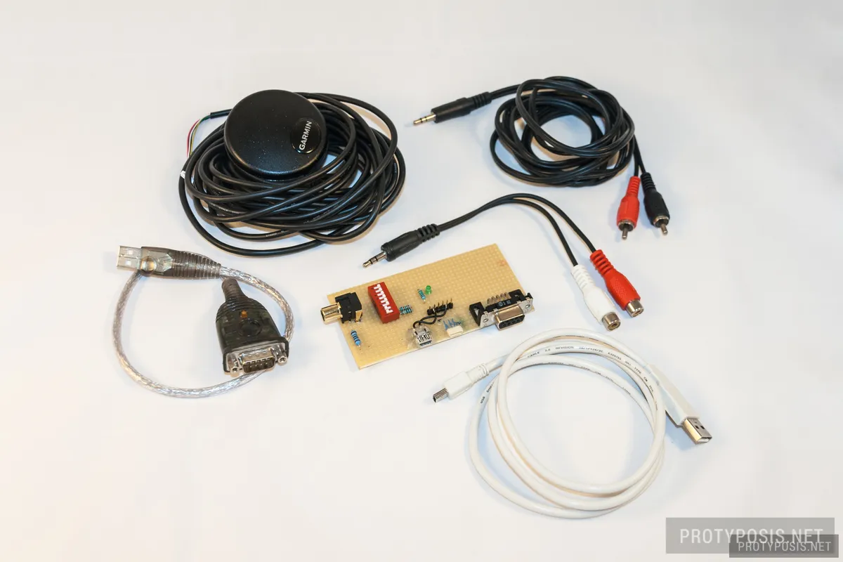
For this guide, we need a desktop PC or laptop running Microsoft Windows, because the software that we are going to use is not available for other platforms. The computer needs an audio interface with a stereo line-in or mic-in, which is available on most desktop PCs. When using a laptop, an additional USB audio interface might be needed, because many new laptops only have a combined headphones + mono mic jack. Of course, using a high quality external audio interface with desktop computers is recommended too. Additionally, you need to get a particular Garmin GPS receiver with a 1 pulse per second output, build an interface board to connect the GPS receiver to the audio input of the computer, and get required cables to connect everything together.
Required hardware:
- Windows computer
- Audio interface with stereo line-in or mic-in
- Garmin GPS 18x LVC receiver
- Interface board (build instructions below)
- USB to mini USB cable (to provide the GPS receiver power)
- RS-232 serial to USB converter (for GPS receiver configuration)
- Stereo cinch cable male (if the audio interface has cinch input)
- Stereo cinch male to 3.5mm stereo male (if the audio interface has 3.5mm input)
- Mono or stereo cinch female to device output (to connect the output of the device to be measured with the male cinch from the audio interface)
The sampling rate of the audio interface is important for the accuracy of the GPS time signal. Most interfaces produced in recent years (even cheap on-board chips) are capable of sampling at 192 kHz, which is recommended. I have also got reasonably good results with 96 kHz sampling. The sampling rate is also important when measuring high audio frequencies, because the maximum measurement frequency is obviously capped by the sampling rate of the audio interface (it is not important for measuring drifts per se, because drift is not dependent on the frequency of the measurement signal).
Setup
Building the Interface Board
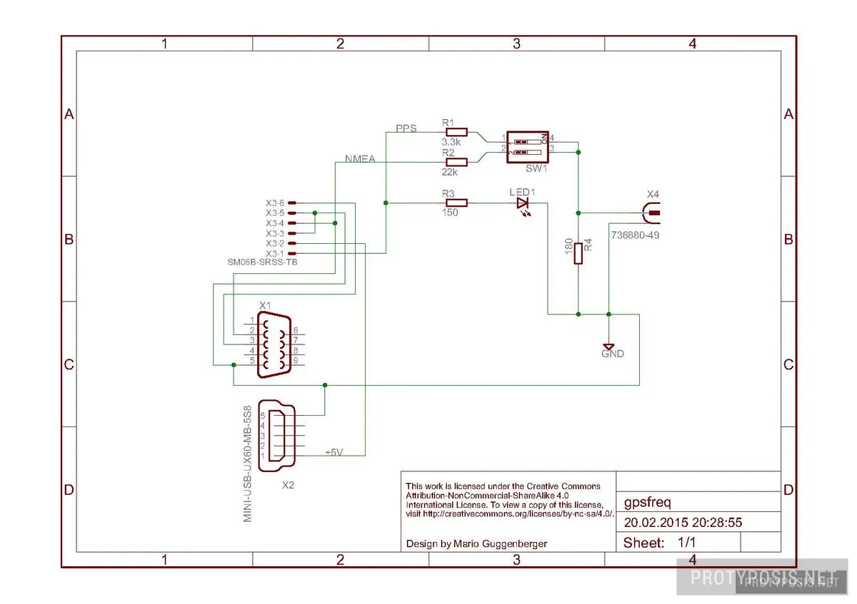
The first step is building the interface board, because we will need it to configure the GPS receiver and later to convert the GPS time pulse signal to an audio signal. The idea of converting the PPS signal to audio level though a simple voltage divider is taken from the Spectrum Lab documentation. This interface board improves this approach by providing all of the following functions on a single and easy to assemble board:
- GPS to audio signal converter
- cinch audio signal output jack (PPS/NMEA audio output)
- GPS receiver port
- PPS notification LED to notify the user of an active signal
- DIP switch to independently enable/disable the PPS and NMEA signals from the GPS receiver
- Mini USB port to power the GPS receiver
- RS-232 serial port to configure the GPS receiver
-
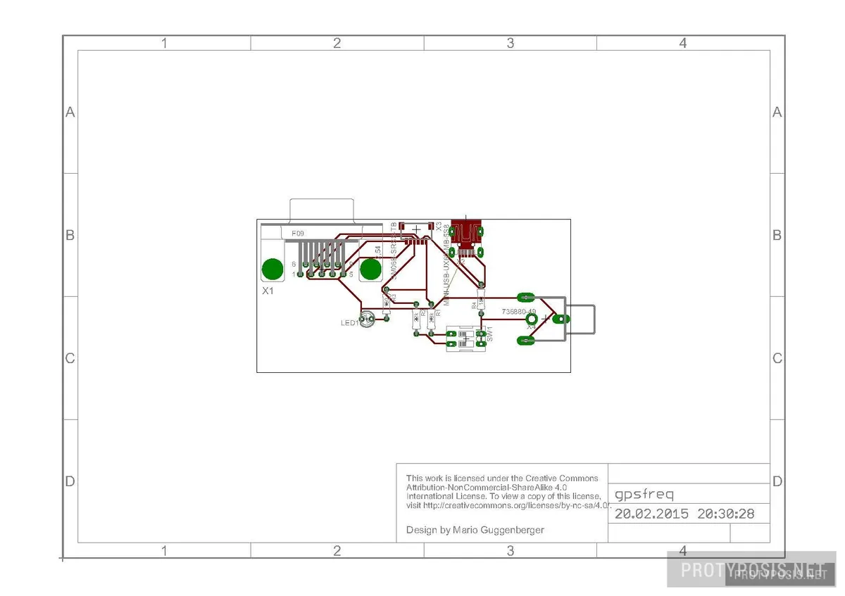
Board layout -
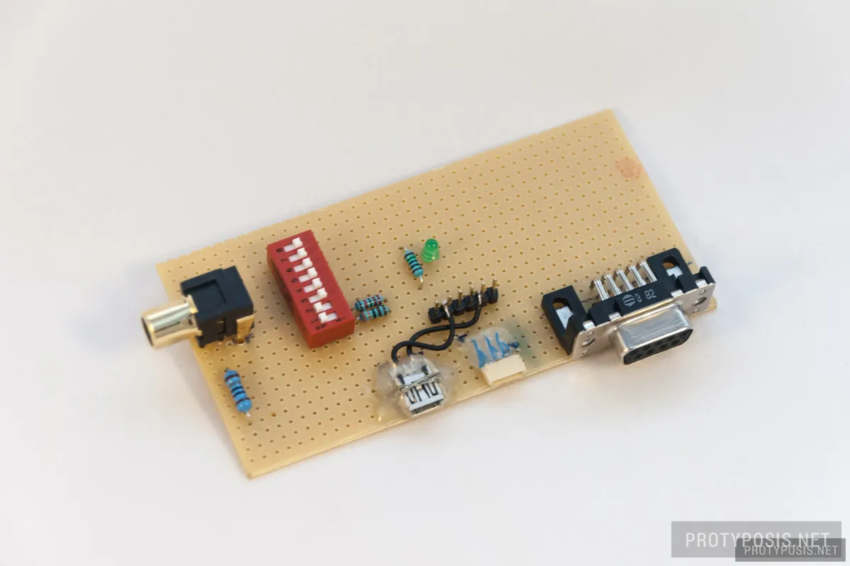
Assembled board (front) -
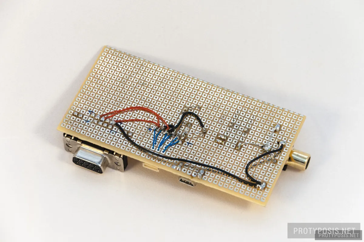
Assembled board (back)
Eagle schematics for building the board are available in the board directory of the repo. The following table lists the required components. Make sure to get surface mount types where possible, ideally with 2.54mm (.1”) pitch pins to fit the perfboard. DIP1 switches the time pulse, DIP2 the NMEA data – this mostly serves to disable NMEA while keeping the time pulse.
| # | Required Parts |
|---|---|
| 1x | perfboard |
| 1x | mini USB type B port (GPS power 5V) |
| 1x | JST SM06B-SRSS-TB (GPS receiver port) |
| 1x | RS232 female port (GPS serial connection) |
| 1x | 3mm LED green |
| 1x | RCA/cinch phono jack (signal output) |
| 1x | 2 pole DIP switch |
| 1x | resistor 150R |
| 1x | resistor 180R |
| 1x | resistor 22k |
| 1x | resistor 3.3k |
Configuring the GPS Receiver
Once the interface board is finished, we can use it to configure the GPS receiver for correct time signal output.
- Connect the GPS receiver to the board
- Provide the board power through the mini USB port
- Connect the serial port of the board with your computer through the RS232 to USB converter
- Download the GPS receiver configuration tool SNSRCFG 3.20 from the Garmin website
- Start SNSRCFG, choose the 18x receiver from the list
- Select Comm > Setup, and choose the correct COM port of the RS232/USB converter
- Select Comm > Connect to connect to the GPS receiver
- Select File > Open… and choose the
SNSRCFG.cfgfile from thegps18xfolder in the repo - Select Config > Send Configuration to GPS to upload the configuration to the receiver
- Select Comm > Disconnect
- Remove the RS232/USB converter. If everything worked as expected, it won’t be needed anymore.
- Power cycle the GPS receiver (disconnect USB power for a moment)
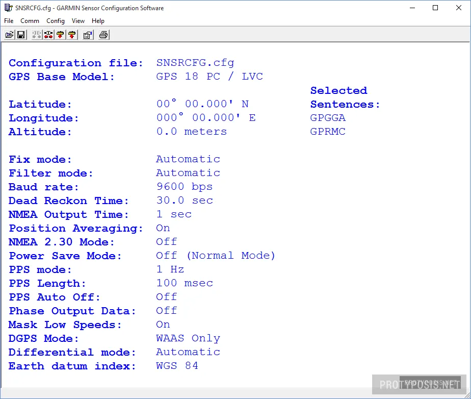
The config file sets the GPS receiver to a serial baud rate of 9600 bps, enables the 1 PPS signal with a length of 100 ms, and disables all NMEA sentences except the two most important ones for this use case. This is not the only possible configuration but this guide will expect it when configuring Spectrum Lab in the next section. If you want different settings, you need to adjust settings in Spectrum Lab accordingly. When selecting additional NMEA sentences, make sure that they fit the interval between the PPS, else the baud rate needs to be increased.
To check for the time signal, place the GPS receiver somewhere with an open view to the sky, ideally outside or directly at an unshielded window. The GPS receiver must be plugged to the board and the board powered through USB. Wait a few minutes until the green LED starts to blink, indicating a PPS signal from the receiver. If it does not start to blink, double check the wiring of the board and that the GPS receiver is positioned correctly.
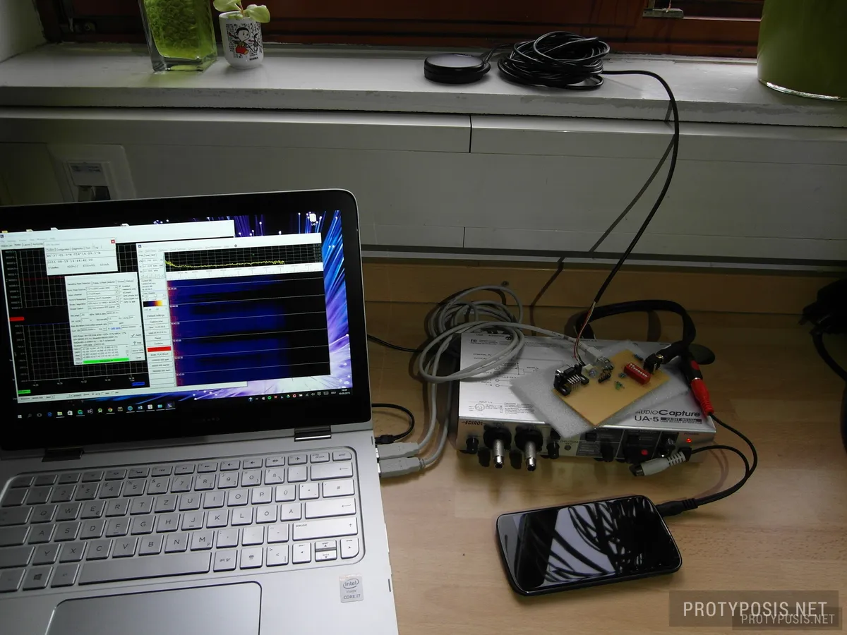
Configuring Spectrum Lab
To complete the setup, we need to connect everything correctly and configure the Spectrum Lab software. The goal of this section is to get Spectrum Lab to pick up the GPS time signal from the left channel of the computer’s audio input and an optional measurement signal from the right channel. Many of the settings are already prepared in a settings file from the repo, so we will just quickly make sure that everything works as expected. Detailed documentation is available in the Spectrum Lab Manual.
- Make sure the board is receiving a PPS signal (check the green LED)
- Connect the cinch output from the interface board to the left input channel of the computer
- Connect an audio source (smartphone/mp3 player/anything that plays music) to the right input channel of the computer
- Download, install and start Spectrum Lab from the website
- Select File > Load Settings From… and open the
DriftAnalysis.usrsettings file from thespeclabfolder in the repo - Resize the main window so you can see all buttons in the left column
- Select Options > Audio Settings to configure the audio input
- Select the correct audio interface from the Input Device dropdown
- Select the same audio interface from the Output Device dropdown
- Select the maximum sample rate that your interface supports from the Soundcard Sample Rate dropdown
- Apply and Close window
- Select Components > Sampling Rate Detector to open the Sampling Rate and Frequency Correction window and check the GPS time signal configuration
- If you get a yellow “Samplerate too far off” warning, your audio interface is already drifted a lot and you need to increase the “Max deviation from initial sample rate” and hit Apply
- Especially when using a mic-in, the input must be levelled correctly. When getting “Sync pulse missing” / “Last sync too old” / “Sync pulses too weak!” / “PPS level too high” errors, the audio input level must be adjusted in the windows audio settings. It should peak between 50% and 100%, clipping must be avoided.
- Everything is OK if you get a green “PPS peaks ok” and regular ppm values in the History box
- Select Show GPS to open the GPS Receiver window and make sure that there is a valid position and at least 1 satellite available (in the lower left corner)
- Close the window
- The sliding spectrogram view in the main window should be empty (black)
- Play some music from the audio source and make sure it comes up in the spectrogram view
When taking measurements, always make sure that you not only get a time signal (green LED blinking), but also that the GPS Receiver window in the Sampling Rate Detector has at least 1 satellite registered. The green LED starts blinking once a valid time pulse from the satellite is available, but continues from the GPS receiver’s inaccurate internal clock generator if the GPS signal is lost, leading to invalid measurements!
The setup process is now complete, and following this guide, everything should be configured and working correctly. It’s finally time to take some measurements!
Measuring Playback Drift
Taking a measurement is very simple. The first time you need to prepare a measurement test audio file with a sine wave of a frequency to your liking, and set this frequency in Spectrum Lab to. Then it is just a matter of playing back this test file and routing the audio output into the right channel input of the audio interface of the measuring computer, and Spectrum Lab displays the measured drift and plots it over time. A few examples: To measure a computer or smartphone, just play back the file with any audio player software (or use a frequency generator program instead of the file). To measure an A/V receiver or TV, put the file on a USB stick or play it over DLNA. Some devices even have a built in test tone functionality that plays a sine wave. On Android devices, you can use my ClockDrift app that is documented here.
The playback drift measurement of a device works by playing back the sine signal with known frequency and setting this frequency as reference in Spectrum Lab. The difference between the expected and measured frequency is the drift shown in units of ppm (parts per million), ms/min, and ms/h.
Sine signal files can be generated with many audio editors and DAWs, MATLAB, or FFmpeg. On smart platforms, there is a range of frequency generator apps available as well which save the intermediary step of generating and transferring a file.
# FFmpeg example: Generating a 10 minute test file with a 440 Hz sine wave
ffmpeg -f lavfi -i "sine=frequency=440:duration=600" testsine440.wav
To take a measurement, make sure Spectrum Lab is correctly configured, and follow these steps:
- Make sure that the sound thread in Spectrum Lab is running, check Start/Stop > Start Sound Thread (this gets disabled by recording drift measurements)
- Prepare the device to be measured with the test file and start playback
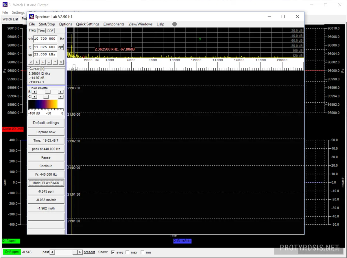
- In the main window of Spectrum Lab, click the red button saying “CLICK TO SET Fr” and type in the reference frequency
- Make sure that the Mode button below says “PLAYBACK”, else click it to switch the mode
- Find the measured drift value below in three different units (pps, ms/min, ms/h)
The measured drift can change over time for various reasons, e.g. power consumption or temperature. To follow it over time, switch to the SL Watch List and Plotter window (or open it through the menu View/Windows > Watch List & plot window). The plotter is already configured to plot the actual sampling rate and drift over time. This window also offers the ability to export the value series to a text file for further analysis or processing in Excel, MATLAB and others (through File > Export to text file).
Measuring Recording Drift
Measuring the recording drift is a bit more complicated. For most devices, measuring only the playback drift is sufficient when the DAC and ADC are part of a single chipset that is driven by the same clock generator, because both drifts will be the same. Still, this is hard to know when treating the device as a black box, and there are devices where it differs.
To measure the recording drift of a device, it needs to record a calibrated test signal, and the recording needs to be analyzed afterwards. To play a calibrated test signal, we can again use our GPS-calibrated Spectrum Lab. When the computer has multiple audio interfaces, make sure that playback goes out through the same audio interface that the time signal comes in, because this is the (only) calibrated interface.
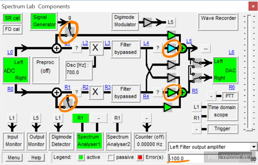
- From the Spectrum Lab main window, select Components > Show Components (circuit window) to open the Spectrum Lab Components window
- Click the Signal Generator box to open the Test Tone Generators window
- In the first line of the Function Generators box, tick “On”, select “sine” waveform, and set your favorite test frequency (e.g. 440 Hz)
- Press the Turn ON button to activate the test tone generator, and the Signal Generator box in the Spectrum Lab Components window turns green
- Back in the Spectrum Lab Components window, we need to setup the circuitry (see the annotated image below for hints)
- Click the DAC box on the right and select “Enabled”. You should now hear the PPS pulse from the GPS through your speaker output.
- Switch the left and/or right channel Signal Generator (g) towards the output DAC by clicking the switches in the grey rectangles (see image). You should now additionally hear the test tone.
- Prevent the input from the ADC passing to the DAC output by clicking the green amplifier triangles in front of the output adders (+) and setting the amplification down to -100 (see image). Now only the test tone should be audible.
You need to do this configuration only once, and can now turn on and off the test tone from the Test Tone Generators window. This does not interfere with the playback drift measurement configuration.
Taking a measurement is now very easy:
- Record the test tone into an audio or video file for some time with the device you want to measure. For a simple measurement sample, a few seconds are enough, but you can record long periods to observe the drift over time. The better the test tone stands out on the recording, the better the quality of the measurement (optimize for high SNR).
- Transfer the recording to your computer
- Convert or extract the audio to an uncompressed wav file (e.g. with FFmpeg:
ffmpeg -i audio_or_video_file.ext -acodec pcm_s16le audio.wav) - Load the wav file into Spectrum Lab or MATLAB (read below for instructions)
Single measurements are best analyzed with Spectrum Lab. Set the reference frequency, switch Mode to “RECORDING”, and load the audio file through File > Audio Files & Streams > Analyze audio file (without DSP) or Analyze and play file (with DSP) if you want to have the measurement plotted over time.
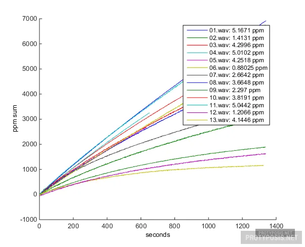
For multiple measurement recordings, there is a MATLAB analysis script in repo. Open the analysis.m file from the matlab folder and follow the inline comments in the script. This script analyzes multiple files and plots their drift over time in a graph.
Measuring Frequency
Because drift is basically a function of frequency, Spectrum Lab is already configured for calibrated audio frequency measurements. Just use Spectrum Lab as it was intended to be used, and consult its manual for further information.
Example Measurements
This is a table of example drift measurements of various devices through this setup or through the ClockDrift app (where indicated).
| Device | Drift (ppm) | Drift (ms/min) | Note |
|---|---|---|---|
| Acer Iconia A200 | +13.39 | +0.80 | audio |
| Acer Iconia A200 | -554.19 | -33.25 | video |
| Acer Travelmate TM8172 | -2.88 | -0.17 | audio / ClockDrift @ Nexus 5 |
| Apple iPad 2 Wi-Fi | +13.73 | +0.82 | audio |
| Apple iPad 2 Wi-Fi | +11.96 | +0.72 | video |
| Apple iPhone 6+ | +416.84 | +25.01 | audio / ClockDrift @ Nexus 5 |
| Apple iPod touch 4G | +416.76 | +25.01 | audio |
| Apple iPod touch 4G | +413.64 | +24.82 | video |
| Asus Nexus 7 2012 Wifi | +2.92 | +0.18 | audio |
| Asus Nexus 7 2012 Wifi | +2.15 | +0.13 | video |
| Asus Nexus 7 2013 Wifi | +7.44 | +0.45 | audio / mean of 8 devices |
| Asus Nexus 7 2013 Wifi | +2.97 | +0.18 | video / mean of 8 devices |
| Canon HF10 | +6.45 | +0.39 | video |
| Edirol UA-5 | -3.21 | -0.19 | audio |
| iRiver H120 | +93.98 | +5.64 | audio |
| iRiver H320 | +57.96 | +3.48 | audio |
| LG Nexus 4 (rev. 10) | +6.74 | +0.40 | audio |
| LG Nexus 4 (rev. 10) | +3.39 | +0.20 | video |
| LG Nexus 4 (rev. 11) | +4.12 | +0.25 | audio |
| LG Nexus 4 (rev. 11) | +1.88 | +0.11 | video |
| LG Nexus 5 | +6.44 | +0.39 | audio / mean of 5 devices |
| LG Nexus 5 | +4.03 | +0.24 | video / mean of 5 devices |
| M-Audio Microtrack 24/96 | -40.42 | -2.43 | audio |
| Samsung Galaxy Nexus | +79.67 | +4.78 | video |
| Samsung Galaxy Note 10.1 | +17.03 | +1.02 | audio |
| Samsung Galaxy Note 10.1 | +13.70 | +0.82 | video |
| Samsung Galaxy S | +4.33 | +0.26 | video |
| Samsung Galaxy S2 | +273.93 | +16.44 | audio |
| Samsung Galaxy S2 | +272.46 | +16.35 | video |
| Samsung Galaxy S3 | +5.67 | +0.34 | video |
| Samsung Galaxy S5 | +1.77 | +0.11 | audio / ClockDrift @ Nexus 5 |
| Samsung Galaxy Spica | -15.13 | -0.91 | audio |
| Samsung Nexus S | -6.17 | -0.37 | video |
| Samsung NP900X3A | -98.25 | -5.89 | audio / ClockDrift @ Nexus 5 |
| Sony PCM-M10 | +8.61 | +0.52 | audio |
| Zoom R16 | +23.46 | +1.41 | audio |
Measurements described in more detail in An Analysis of Time Drift in Hand-Held Recording Devices.
Troubleshooting
- When not getting a time signal, check the DIP switches and the audio input settings.
- If the plotter graph is garbled, enter the “Plotter” menu and select “Refresh Display”.
- If the spectrogram does not advance and the Sampling Rate Detector does not work either, check if the sound thread is running in main menu Start/Stop > Start Sound Thread. This happens after analyzing a file.